Journey to Zero-Knowledge
Created:
2023-08-06
Updated:
2023-12-26
Introduction
Zero-Knowledge Proofs (ZKP) represent a fascinating and influential concept within the realm of cryptographic protocols.
At a glance, a ZKP enables one party to demonstrate the correctness of a statement to another party without revealing any details beside the validity of the claim itself.
ZKPs find applications in various areas, including secure authentication protocols, blockchain systems, and secure computation, among others.
Another motivation is philosophical. The notion of a proof is basic to mathematics and to people in general. It is a very interesting and fascinating question whether a proof carries with it some knowledge or not.
In this paper we incrementally construct a path leading from the classic mathematical notion of proof to those that share zero knowledge. One of the goals is to demystify the subject, maintaining the necessary rigor while ensuring accessibility for a broader audience.
Classical Proofs
Deductive Reasoning
Deductive reasoning is a fundamental method of logical thinking used across various disciplines, from philosophy and mathematics to computer science and law.
It involves deriving specific conclusions from a set of general premises or known facts. The strength of deductive reasoning lies in its ability to guarantee the truth of the conclusion, provided the premises are true, and the reasoning process is logically sound.
One of the earliest examples of deductive reasoning can be traced back to ancient Greek philosophers, particularly Aristotle, who formalized the syllogistic reasoning. A classic example of a syllogism is:
- All men are mortal (premise).
- Socrates is a man (premise).
- Therefore, Socrates is mortal (conclusion).
This example captures the essence of deductive reasoning: if the premises are true and the reasoning is valid, then the conclusion must also be true.
Deductive Reasoning in Mathematics
In the realm of mathematics, deductive reasoning takes on a more structured form known as a mathematical proof.
A mathematical proof is a logical argument presented systematically to verify the truth of a mathematical statement. Here, deductive reasoning is used to derive conclusions from a set of axioms (self-evident truths) and previously established theorems (proven statements) by using some inference rules which can be applied in the specific context.
By setting the conclusion as the statement we want to prove and the premises as the set of axioms and previously proven theorems, we can define a proof as a finite length string encoding the set of logical derivation that incrementally drives from the premises to the conclusion.
As all the proof reasoning rely on the basic properties of boolean algebra, it is implicit that Boolean logic axioms and theorems holds as premises for any reasonable proof systems which we’ll analyze in the context of this document.
Validity and Soundness
A proof is valid if the conclusion logically follows the premises, regardless of whether those promises are true or not.
A proof is sound if is valid and all of its premises are true.
Example. Sound proof.
-
Premises:
A,BandCare three sets such thatA ∩ B ⊆ C;x ∈ B;- basic properties of set theory hold;
-
Conclusion:
x ∉ A \ C. -
Proof:
x ∉ A \ C = ¬(x ∈ A ∧ x ∉ C) = x ∉ A ∨ x ∈ C = x ∈ A → x ∈ CA ∩ B ⊆ C ∧ x ∈ B ∧ x ∈ A → x ∈ C
Example. Valid but not sound proof:
- Premises:
- All prime numbers are odd (wrong premise).
- 2 is a prime number (as it has no divisors other than 1 and itself)
- Conclusion: 2 is odd
- Proof: The conclusion follows directly from premises.
As you can see, since the conclusion can be derived from the premises, the proof is formally correct, but as the second premise is not incorrect it is not sound.
The example emphasize how we can reach incorrect conclusions even though we constructed an apparently correct proof just because of a bad premise.
Proof Systems
A proof system is a formal and systematic (algorithmic) approach to construct and evaluate proofs.
It typically consists of the following key components:
-
Statement (x): assertion under consideration. It is the proposition that one tries to prove or disprove.
-
Proof (π): set of arguments, evidence, or logical steps that, when processed by the proof system, should establish the validity of the statement.
-
Prover (
P): algorithm to construct a proof for the given statement (P(x) = π). -
Verifier (
V): algorithm that, given both the statement and the proof, decides whether the proof is valid. This algorithm outputs1if the proof is correct and0if the proof is not correct (V(x,π) = 0|1).
Clear rules and guidelines are essentials when we need to move proof construction and checking from the often ambiguous and nuanced domain of natural languages to the precise realm of formal languages.
Though this discussion, we’ll mostly adhere to the popular convention of referring to the prover as Peggy and the verifier as Victor.
Knowledge Sharing
In a classical proof system a proof that some assertion is true inherently reveals why it is true. This aspect is deeply bound with how the classical mathematical proof systems works: Peggy shares all the logical steps to allow Victor to independently reach the same conclusion.
Follows that the proof provides more knowledge than just the mere fact that the statement is true, which is what Peggy and Victor are interested in the first place, regardless of the way this is proven.
For instance, consider the task of proving knowledge of the factorization of
a natural number n, Peggy could simply provide the list of its prime factors
{pᵢ}. Victor can efficiently check if n = ∏ᵢ pᵢ. In the end, not only
Victor is convinced about our statement, but he also gains knowledge the
factorization of n.
The information which facilitates the construction of the proof is known as the witness. In a classical proof system, sharing the witness with the verifier equates to providing a standard proof. However, if the witness remains confidential, the proof is known as a Zero-Knowledge (ZK) proof.
Formalization and Relationship to Complexity Theory
As proof systems transition into the domain of computational machines, it becomes crucial to define a non-ambiguous method for analyzing their complexity, including the resources required for proving and verifying the problems.
Find a clear relationship between proof systems and important complexity classes,
such as NP, is essential for understanding the tractability of some problems
in terms of proof construction and verification.
In computational theory, problems are often associated with languages over specific alphabets. This association helps to formalize and understand the range of problems that computers can solve.
Many interesting problems are formulated as decision problems, where the answer is either true or false. These problems can be associated with languages where strings represent instances of the problem, and membership in the language indicates a positive answer (true), while non-membership indicates a negative answer (false).
Consider the Subset Sum Problem (SSP) as an example. The core question is
whether there is a subset of integers that adds up to a target t.
The problem can be represented as the language:
L = { x = (S,t) | S ⊆ ℕ and ∃ V ⊆ S: sum of elements in V equals t }
In this language, a pair x = (S,t) (a string) belongs to the language L
if and only if satisfies the language condition, i.e. there is a subset of S
which adds up to t.
Key characteristics of proof system (P,V) for decision problems:
- Completeness:
x ∈ Lif and only ifV(x,π) = 1; - Soundness:
x ∉ Lif and only ifV(x,π) = 0; - Efficiency:
V(x,π)runs in polynomial time with respect to length ofx.
Since each problem belongs to a complexity class, once we mapped the problem
to a language, we implicitly associated the language to the same complexity
class. For instance, a language L belongs to NP if a solution to the
problem associated to L can be verified by a deterministic Turing machine
in polynomial time, even though finding the solution itself (constructing the
proof) may be a way more computationally intensive task.
Interactive Proofs
An interactive proof (IP) system extends the classical notion of proof system by transitioning from a proof conceived as a static sequence of symbols to an interactive protocol where Peggy incrementally convinces Victor by actively exchanging messages.
The concept was first proposed in the mid-1980s by Goldwasser, Micali, and Rackoff in their seminal paper “The Knowledge Complexity of Interactive Proof Systems” [GMR]. Their work not only introduced interactive proofs but also presented the first formal definition of zero-knowledge proofs.
Is worth noting that Babai [BAB] independently contributed to the development of this field approximately during the same period with his paper “Trading Group Theory for Randomness”.
In IP systems, the complete ordered sequence of messages exchanged during the protocol is referred to as the transcript. Two runs of the same protocol can result in different transcripts. This variability depends on whether the protocol is deterministic or probabilistic.
Sigma Protocols
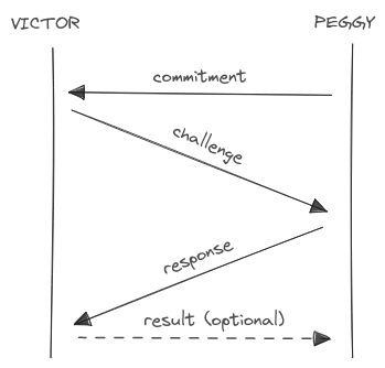
Any IP system with a transcript composed of four messages is called a sigma protocol.
The name of the protocol is inspired by the Greek letter Σ, which shape
mirrors the sequence of the protocol’s steps:
- Commitment: Peggy initiates the protocol by sending the first message.
- Challenge: Victor responds by issuing a challenge to Peggy.
- Response: Peggy replies to the Victor’s challenge.
- Result (optional): Victor sends a message with the verification outcome.
The names of these steps were chosen to reflect their functional roles in the execution of typical proofs, particularly in the ZK context. For the moment the detailed mechanics and purpose of each step are left open.
This type of protocols is the most widespread when comes to ZKP, indeed every protocol which will be analyzed in the ZKP examples section is a sigma protocol.
For completeness, note that some sources describe sigma protocols with just three messages, excluding the optional fourth “result” step.
Deterministic Interactive Proofs
A deterministic IP is an interactive proof which doesn’t introduce any
randomness in the protocol messages. In such a system, Victor asks questions and
Peggy is expected to always reply with the same answers.
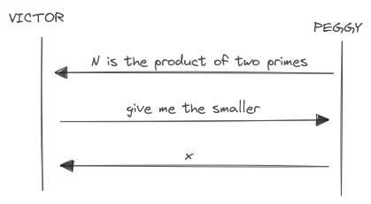
As an example, consider the protocol where Peggy wants to prove that she knows that a number is the product of two primes.
Using a transcript similar to the sigma protocol:
- Commitment: Peggy asserts she knows the factors of a number
N. - Challenge: Victors asks for the smaller (or the bigger) factor.
- Response: Peggy sends the smaller (or the bigger) factor.
- Result (optional): Victor accepts or reject.
The verification of the proof is quite simple and fast:
- compute
y = ⌈N / x⌉ - check if
N = x·y - check if both
xandyare primes via some deterministic algorithm (can’t use a probabilistic algorithm as the verification result should be deterministic).
Every deterministic
IPcan be trivially mapped into a static classic proof and vice versa.
To convert a static proof into a deterministic IP, the two parties can just
communicate to incrementally transfer one or more chunks of the proof. Note that
a static proof is essentially a deterministic IP with a single message exchange.
This mapping is not very interesting.
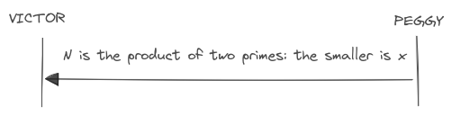
To convert a deterministic IP to a static proof is sufficient for the prover
to construct a single string encapsulating the entire protocol transcript. This
construction is feasible because of the deterministic nature of the transcript,
where every message sent by Victor is predictable. Victor, just have to check if
the set of messages in the transcript is consistent with the expected ones.
From this last result follows that deterministic IP systems are not more
powerful than static proofs with respect to the set of languages that can be
proven.
Due to the limited interest in deterministic IPs, we will save formal
definitions for the next chapter.
Probabilistic Interactive Proofs
In the probabilistic version of the proving system, the steps mirror those of the deterministic counterpart, but with additional elements of randomness introduced by either the prover, the verifier, or both.
The introduction of randomness into the protocol can, in some scenarios, lead to more efficient proofs or enable to prove en entire new class of languages which can’t be proven using deterministic proof systems.
As outlined by GMR:
- Peggy is assumed to have unbounded computational resources, while Victor operates within polynomial time constraints relative to the size of the statement to prove.
- Given Victor’s polynomial computational limitations, the number of messages exchanged between the two must also be polynomial.
- Both Peggy and Victor have access to a private random generator.
Formally:
A probabilistic
IPsystem for a languageLis a protocol(P,V)for communication between a computationally unbounded machinePand a probabilistic polynomial time machineVtaking an input statementx, a message history (hᵢ) and randomness source (r) to produce the next protocol message:
m₁ = V(x, rᵥ, h₁={})
m₂ = P(x, rₚ, h₂={m₁})
m₃ = V(x, rᵥ, h₃={m₁,m₂})
...
As a shortcut, from now on we’ll refer to probabilistic interactive proof
systems just as interactive proof (IP) systems.
Key characteristics of an IP system (P,V) for a language L:
- Completeness: If
x ∈ L, thenV(x,π) = 1with probability at least1-ε. - Soundness: If
x ∉ LthenV(x,π) = 1with probability at mostε. - Efficiency: Both the total computation time of
V(x,π)and the overall communication in(P,V)is polynomial with respect to length ofx.
The parameter ε represents a cap on the verifier’s error probability,
an is popularly known as the soundness error.
If for a single protocol execution ε < 1, then we can always derive another
protocol which executes the original one k times consecutively, thus
exponentially reducing the error probability to an arbitrary value εᵏ.
For instance, if ε = 1/10, executing the protocol 5 times would reduce the
error probability to ε⁵ = 1/100000, allowing Victor to accept with a
probability of 0.99999.
Constructing a static proof for some problems can be significantly more challenging. This is partly because the prover has to answer in advance to all the possible questions from Victor and encapsulate all the potential Peggy’s responses in one single message. This is not always possible given the polynomial nature of the verifier.
As we’ll see later, there is an entire class of problems which cannot be practically proven via static proofs.
Proving Completeness
Completeness is quite easy to prove.
If Peggy knows the solution to a problem, she will eventually convince Victor
as its responses during the repeated protocol executions will be always correct
regardless of the number of repetitions and the value of ε.
Proving Soundness
Soundness is a bit more challenging to prove.
A proper proof of protocol soundness generally requires an extractor, a hypothetical tool tailored for the specific protocol which allows Victor to extract key information used by Peggy to construct the proof.
Imagine Victor being capable of rewind Peggy’s execution without her knowledge. In such a case, Peggy would re-execute the protocol exactly as before, even using the same random values as in the previous execution. From Peggy’s perspective, these executions would appear statistically indistinguishable.
If under these conditions Victor is able to recover some information which allows him to construct a valid proof then the protocol is sound.
The intuition here is that it is statistically impossible for a dishonest Peggy to disclose crucial information without actually possessing it. Should would require an extraordinary stroke of luck to fabricate this information out of thin air.
It is important to note that the extractor is a theoretical construct, not meant to be present in any real-world execution of the protocol. For example, if the environment is the real world, it could be something like a time machine. In the digital world, it could be the capability to snapshot and restart the prover state at any point.
Interactive Turing Machines
Let’s invest some time formalizing a bit further the execution environment for the interactive proofs, i.e. the interactive proof system.
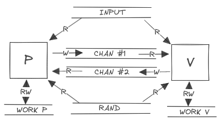
An Interactive Turing Machine (
ITM) is a Turing machine with a read-only input tape, a read-write work tape, a read-only random tape, a read-only communication tape and a write-only communication tape.
In an IP system, both the prover (P) and the verifier (V) are defined
as ITM who share the same input tape, which generally contains the encoded
assertion to be proven.
The read-only communication tape of one machine is defined to be the write-only communication tape of the other machine. This type of tape is used to exchange protocol messages.
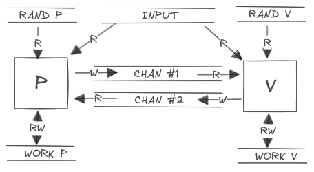
During the proving protocol, the two machines take turns in being active.
With each protocol step, the ITM utilizes all its readable tapes as inputs
for internal computations. It then writes the resulting output to the write-only
communication tape (which corresponds to the read-only input of the other
machine).
The final message of every reasonable protocol goes from P to V, which can
then accept or reject the proof.
Consistent with our earlier discussions, P is considered to have unlimited
computational resources, while V operates under a computational constraint,
which are polynomially bounded by the size of the assertion being proved.
Interactive Proof Computational Complexity Class
In this section, we give a small insight about the complexity class associated
with IP systems. This topic is highly theoretical and falls somewhat outside
the primary focus of this document.
The
IPcomplexity class is defined as a class of languages for which there exists anIPsystem whose proofs can be verified in polynomial time with respect to the length of the statement to prove.
IP = { L | L has an interactive proof }
This class can be further divided based on the protocol’s characteristics. For
instance, IP[k] denotes the class of languages that can be decided by an
interactive proof with k rounds.
At the beginning of the 90s, Lund, Fortnow, Karloff and Nisan [LFKN]
proved that PH ⊂ IP, which shows that interactive proofs can be very powerful
as they contain the union of all complexity classes in polynomial hierarchy
(PH), including P, NP, co-NP.
Shortly later, Shamir [SH] proved that in fact IP = PSPACE, which gave a
complete characterization of the capabilities of interactive proofs.
As a direct outcome, employing an interactive proof system enables to verify
solutions for problems that fall outside of NP and even beyond the scope of
PH.
In some cases, the interaction between Peggy and Victor can also lead to a more
efficient verification process, allowing Victor to accept a proposed solution
without the need for Peggy to share the entire solution (ZK proofs).
Arthur-Merlin Protocols
An Arthur-Merlin protocol,
initially introduced by Babai [BAB] in 1985, is an IP system with the
additional constraint that the prover and the verifier share the same
randomness source.
In this context, Merlin is the prover, Arthur is the verifier and both of them are allowed to see the randomness source of the other party.
The fundamental attributes of an AM proof system (P,V) for a language L,
such as completeness, soundness, and efficiency, align with those of
general IP systems.
MA Protocols
The set of decision problems that can be verified in polynomial time using a
single message AM protocol forms the MA set.
Steps for a generic MA protocol:
- Merlin sends to Arthur the proof.
- Arthur decides.
MA protocols are very similar to traditional NP proofs with the addition
that the prover can use a public randomness source to construct its proof.
AM Protocols
The set of decision problems that can be decided in polynomial time by an AM
protocol with k messages is called AM[k].
For all k ≥ 2, AM[k] is equivalent to AM[2]. This result is due to the
fact that Merlin can observe Arthur randomness source during the whole
protocol execution, and thus it doesn’t affect Merlin messages.
MA is strictly contained in AM, since AM[2] contains MA but AM[2]
cannot be reduced to MA
Goldwasser and Sipster [GS] proved that for any language with
an interactive proof protocol with private randomness (IP) also have an
interactive proof with public randomness (AP). In particular, for any k:
AM[k] ⊂ IP[k] ⊂ AM[k + 2]. And since AM[k + 2] = AM[k] = AM[2] follows
that IP[k] = AM[2].
In short, any language with a k-round private coin IP system has a
k = 2 round public-coin AM system.
Said that, is worth anticipating that even though general IP systems with
secret random source are not more powerful in terms of the range of languages
they can prove, the secrecy of the randomness becomes crucial for proving
statements without sharing any knowledge.
Examples
Tetrachromacy
Tetrachromacy is a condition enabling some individuals to perceive a broader spectrum of colors than the typical trichromat, who has three types of cone cells for color vision. Tetrachromats have an additional cone cell type, allowing them to see a wider range of colors.
In this scenario, Peggy claims to be tetrachromat and wants to prove it to Victor by showing that she’s able to distinguish between two marbles who appear identical to Victor.
Protocol:
- Peggy places the two marbles in from of Victor and turns her back.
- Victor flips a coin. Based on the outcome, he may swap the position of the marbles.
- Peggy, facing the marbles again, tells Victor whether their positions were swapped.
The likelihood of Peggy falsely claiming to distinguish the marbles and being
able to cheat (soundness error) is ε = 1/2. By repeating this protocol k
times, the probability of Peggy cheating reduces to 1/2ᵏ.
Note that in this protocol a malicious Victor may put another, apparently equal, marble in front of Peggy and infer if that is equal or not to the other.
Quadratic Non-Residuosity
A number y ∈ Zₘ* is a quadratic residue if there exists an x ∈ Zₘ* such that
x² ≡ y (mod m). If no such x exists, y is a quadratic non-residue modulo m.
We define the languages:
QR  = { y | y ∈ Zₘ* and is a quadratic residue }
QNR = { y | y ∈ Zₘ* and is a quadratic non-residue }
It is considered to be a hard problem to tell if y ∈ QR or y ∈ QNR without
knowing the factorization of y.
Notice that both QR and QNR languages belong to NP, and thus they have
a classic proof system: Peggy just needs to send to Victor the factorization of
y without any further interaction.
If instead the prover wants to prove that y ∈ QR or that y ∈ QNR without
sharing the factorization of y this is actually possible only via an IP
system.
A protocol to show that y ∈ QNR is based on the fact that if y ∈ QNR then
y·k² ∈ QNR for any k ∈ Zₘ*.
Protocol [GMR]:
- Victor selects a random number
r ∈ Zₘ*and flips a coin. If the coin shows ‘heads’ he setst = r² mod melset = y·r² mod m. He sendstto Peggy. - Peggy, which has unrestricted computing power, finds if
tis a quadratic residue (i.e. ift = r² mod m) and tells Victor what was his coin toss result.
If y ∉ QNR then y ∈ QR and thus, regardless of the coin toss result,
t ∈ QR as well. In this case Peggy has no way to recover the coin toss
results. In fact Peggy has ε = 1/2 probability of guessing correctly.
As usual, the soundness error probability can be arbitrarily reduced by performing multiple protocol runs.
Note that in this protocol Peggy also reveals some extra information.
If y ∈ QNR a malicious Victor can send to Peggy any number k and learn from
the response if k ∈ QR or not.
As we’ll see in the next sections we can prove both y ∈ QR or y ∈ NQR
without sharing any information using an interactive zero knowledge proof.
Zero Knowledge Proofs
Now that we defined the interactive class of proof system is finally time to better discuss the core topic of this lecture: the quantity of knowledge required to validate a statement.
The concept of Zero-Knowledge Proofs (ZKP) was first rigorously defined in the 1980s by Goldwasser, Micali, and Rackoff in their seminal paper [GMR] (notably, the same paper that introduced Interactive Proof systems).
Before the GMR paper, most of the effort on IP systems area focused on
the soundness of the protocols. That is, the sole conceived weakness was a
malicious Peggy attempting to trick Victor into approving a false statement.
What Goldwasser, Micali and Rackoff did was to turn the problem into: what
if instead Victor is malicious?
The specific concern they raised was about information leakage. Concretely, how much extra information is Victor going to learn during the execution of the protocol beyond the mere fact that the statement is true.
In the realm of ZKP, the primary goal of Peggy is thus to convince Victor that
a certain fact is true, without revealing any additional information.
Naively, it might seem that any additional information in a proof only
pertains to the specific details regarding the how and why the statement
being proven is true. However, the criterion in ZKP is more stringent. It
encompasses any piece of information that Victor cannot independently compute,
extending even to facts that are not directly related to the proof itself.
More formally.
Definition. A proof system for a language
Lis zero-knowledge if, for allx ∈ L, Peggy reveals to Victor only the fact thatx ∈ L(i.e., a single bit of information).
This definition holds true even when Victor is not honest, bounded by his polynomial-time capabilities.
Key attributes of a ZKP system (P,V) for a language L:
- Completeness: If
x ∈ LthenV(x,π) = 1with high probability. - Soundness: If
x ∉ LthenV(x,π) = 1with negligible probability. - Efficiency: The total computation time of
V(x,π)and total communication in(P,V)is polynomial with respect to length ofx. - Zero-Knowledgeness: The proof does not reveal any additional information other than the fact that the statement is true.
Of most importance is the following result found in the [GMW] paper:
Theorem. For any problem in
NPthere exist aZKPsystem.
The theorem is the sweet consequence of the existence of a ZKP system for
the graph three coloring problem, which is known
to be NP complete.
Proving Zero-Knowledgeness
The proof is based on the existence of a simulator and the idea is quite similar to the one used to prove soundness with the extractor.
A simulator is a hypothetical tool which allows Peggy to convince Victor that a statement is true, and thus about the knowledge of some key information, when in reality she doesn’t possess any knowledge.
The key intuition here is that if Peggy can consistently convince Victor of the statement’s truth across multiple protocol rounds without any actual knowledge, then the protocol itself can’t reveal any information to Victor. In essence, Victor cannot discern whether Peggy truly holds any knowledge based on the protocol’s execution.
Similarly to the extractor, the implementation of the simulator is based on rewinding Victor’s execution in order to gain some advantage without him noticing.
From Victor’s perspective, the outputs produced by the simulator are statistically indistinguishable from any genuine protocol execution.
Probability Distributions Distinguishability
Distinguishability refers to the ability of a polynomially computationally bounded Turing machine to distinguish between two random variables.
In the realm of cryptographic protocols, ensuring indistinguishability between different protocol paths or choices is key to maintaining security against adversaries.
In particular, in ZKP protocol, indistinguishability is relevant to ensure that during the protocol execution no information is leaked by the prover and thus the property is carefully evaluated when analyzing the protocol zero-knowledgeness property and thus when constructing the simulator. The verifier should not be able to distinguish between the real prover and the simulator responses.
More formally, consider two families of random variables, P and S, defined
over a language L ⊆ {0,1}*. Indistinguishability of these variables becomes
significant in scenarios where a verifier must decide whether a given sample
originated from P(x) or S(x) for some x ∈ L.
The verifier’s decision-making process is influenced by two factors:
- The size of the sample.
- The time available to decide.
Based on these parameters, P and S can be classified as:
- Equal: if the decision is random regardless of time and sample size.
- Statistically indistinguishable: if the verdict becomes random when given
infinite time and samples with polynomial size with respect to
|x|. - Computationally indistinguishable: if the verdict becomes random when both
time and samples size are polynomially bounded by
|x|.
In practice, given the verifier polynomial bounds, practical ZK proofs are often concerned with computational indistinguishability
Additional Considerations
Any ZK protocol must be run in an environment which preclude the feasibility
of constructing either an extractor or a simulator. The existence of these
tools fundamentally compromise the proof’s soundness and zero-knowledgeness.
If Victor is able to construct an extractor then it will be able to extract knowledge from the proof, and thus undermine zero-knowledgeness. Conversely, if Peggy is able to construct a simulator she will be able to forge valid proofs without any knowledge, and thus undermine soundness.
Since re-playing a protocol breaks the fundamental properties, we can’t use a recording of the protocol execution to convince a third party about the authenticity of a proof. Such a party has no way to tell if the recorded execution is genuine or if the protocol steps were edited (which in practice is a way of rewinding the execution).
Follows that in the context of a ZKP system Peggy is able to convince only the
verifier who actively participates by executing the protocol interactively and
in real-time.
This limitation is often regarded as a feature of some ZKP systems and indeed reflects the pure definition found in the original paper.
Commitment Protocols
In all the ZK protocols discussed in this paper, the only overarching
cryptographic required tool is a commitment protocol so we thing a short
glimpse to the topic is necessary.
This protocol consists of two phases:
- Commit Phase. During this phase, the sender commits to a certain value
vwithout revealing its details to the receiver. Crucially, the receiver should not be able to determine anything useful aboutv. - Reveal Phase. Later on, the two parties may perform a reveal phase,
where the receiver learns the value of
v. There should only one value ofvwhich is compatible with the committed value.
Given H a cryptographically secure hash function, a very simple commitment
scheme for a value x is to share the value c = H(x). To open the commitment
the value of x is revealed. This is secure under the assumption that the hash
function is secure.
Both the computational complexity and the communication complexity of such protocols are reasonable and in fact one can amortize the work if there are several simultaneous commitments.
Simple ZK Protocols
While real-world ZK proofs often rely on intricate mathematical structures and cryptographic techniques, there are intuitive examples that effectively convey the same core principles of ZK proofs.
Except where specifically indicated, the protocols discussed are both sound and zero-knowledge. This is because it is feasible (and often straightforward) to construct both an extractor and a simulator for them.
Where is Waldo
“Where is Waldo?” is a famous kid’s puzzle where, given a very detailed illustration with many different characters the goal is to find Waldo, the main character.

Peggy asserts she knows where Waldo is and should convince Victor without revealing any additional information.
Protocol [NR]:
- Peggy covers the illustration with a large sheet of paper (bigger that the one with the illustration) which has a little hole in the center, positioned exactly over Waldo’s face.
- Victor is convinced if he sees Waldo through the hole.
However, this initial protocol does not adequately address soundness concerns. How can the verifier be sure the covered illustration is the original one?
The following extended protocol is designed to be sound:
- Peggy covers the illustration with a bigger sheet with a randomly positioned hole, then it covers this with an even bigger sheet without any hole. The illustration should be at a distance from the border at least equal to the size of the first sheet of paper (to better hide relative positions during the proof).
- Victor flips a coin and depending on the outcome, asks to Peggy either the removal of both layers to reveal the full illustration or just the top layer to reveal Waldo through the hole.
- Peggy complies with the challenge.
- Victor is convinced based on the evidence.
For one run, soundness error is ε = 1/2, meaning that Peggy has a 50% chance
to cheat.
A similar technique will be used in most of the subsequent protocols. Once Peggy committed the illustration position in the initial step, she can’t change it. Since she doesn’t know if Victor will ask her to reveal the original illustration or the face of Waldo, she must be prepared to satisfy either of these potential demands.
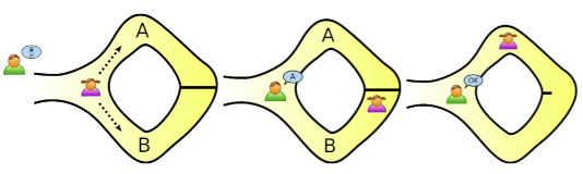
Ali Baba Cave
The story is about Ali Baba, a guy who knows the magic spell to open a secret door in a cave. The cave has a single entrance and splits into two paths, which reconnect at the end through this magic door. Ali Baba can prove his knowledge of the spell without revealing it.
Protocol [QUI]:
- Ali Baba enters the cave and randomly takes one of the two paths, while Victor waits outside.
- Victor enters the cave, goes to the bisection, flips a coin, and based on the outcome, asks Ali Baba to come out from a specific path.
- Ali Baba complies with the Victor’s request, using the magic door if necessary.
- Victor is convinced or not based on the evidence.
For one run, soundness error is ε = 1/2.
It is worth noting that if both parties go to the cave entrance together, Victor
can observe Ali Baba entering one path and exiting from another, confirming
his knowledge in one single run (ε = 0). However, this approach doesn’t align
with the pure definition of ZK proof which should be tailored to convince only
Victor. The possibility of third parties observing or Victor recording the event
would extend the proof’s validity beyond the intended verifier.
Intermediate ZK Proofs
Sudoku
Given a Sudoku puzzle instance, Peggy wants to convince Victor that she knows the solution without revealing it.
Protocol [GNPR]:
- Peggy places three cards on each cell of the Sudoku grid. Pre-filled cells she places three cards with the assigned value, face-up. For other cells, she places the cards according to the solution, face-down.
- Victor randomly selects one of the three cards from each cell across every row, column and subgrid, creating 27 groups of cards.
- Peggy shuffles each group independently, and gives the shuffled groups to Victor.
- Victor checks that each group contains all numbers from 1 to 9.
The soundness error for this protocol is ε = 1/9 (refer to [GNPR pp.~9] for
a proof).
The puzzle can be easily expressed as a graph coloring problem. For example,
3²⨯3² variant is mapped to a graph with 81 vertices, one vertex for each cell.
The vertices are labeled with ordered pairs (x,y), where x and y are
integers between 1 and 9. Two distinct vertices labeled by (x₁,y₁) and
(x₂,y₂) are joined by an edge if and only if:
x₁ = x₂(same column) or,y₁ = y₂(same row) or,⌈x₁/3⌉ = ⌈x₂/3⌉and⌈y₁/3⌉ = ⌈y₂/3⌉(same3⨯3subgrid)
A valid solution assigns an integer between 1 and 9 (the color) to each
vertex, such that vertices that are joined by an edge do not have the same
integer assigned to them.
Graph Three Coloring
The generic graph coloring problem is about deciding if a given graph vertices can be colored such that no two adjacent vertices share the same color.
Given a graph Peggy wants to convince Victor that she knows the solution for the graph three coloring problem for it, which is a specialization of the generic problem which only three colors are allowed.
Protocol [GMW]:
- Peggy draws the graph, assigns to the solution the colors randomly and covers each vertex with a hat.
- Victor randomly selects two adjacent vertices and aks Peggy to reveal their colors.
- Peggi reveals the colors of the selected vertices.
- Victor accepts or reject the proof based on the evidence.
Given E the number of edges in the graph, since Victor checks only one out of
the E possible ones, the soundness error probability is ε = (E-1)/E.
The error approaches to 1 quite fast with the number of edges. Even though this
value can be reduced arbitrarily by repeating the protocol, it is also quite
expensive to be performed in practice.
For example, if E = 1000 and the verifier wants ε < 0.1 then the protocol
should be iterated for k rounds where (999/1000)ᵏ < 1/10 and thus k > 2301.
However, from a theoretical point of view this problem is quite important as it
is an NP complete problem, which means that we can construct a ZK proof for
any problem in NP.
You can find a nice app showing this proof in action here.
Proofs for all NP
While the examples provided in this section might seem limited in their direct
application both are solutions for NP-complete problems.
The implication is profound: any problem in the NP class can theoretically
be converted into an instance of the graph three coloring, and thus a ZKP
exists for every problem in NP.
The typical method for such a transformation begins with reformulating the NP
problem into a Boolean circuit. This circuit is designed to generate a true
output if and only if the input represents a correct solution to the original
NP problem. Subsequently, this Boolean circuit is converted into a graph.
The construction of this graph ensures that finding a valid three-coloring
correlates directly with solving the original NP problem.
While theoretically feasible, this approach is often not practical. The
transformation process can be computationally expensive, not to mention the
high soundness error of the graph three coloring problem. Therefore, in
practice, where possible more specialized and efficient approaches are employed
for specific NP problems.
More Advanced ZK Protocols
Graph Isomorphism
Two graphs G₀ and G₁ are isomorphic if a bijective mapping f: G₀ → G₁
exists such that for any edge (v,w) in G₀ there is a corresponding edge
(f(v),f(w)) in G₁.
The problem about determining if two graphs is known to be in NP, but at the
current state of knowledge, not NP-complete.
For this problem, Peggy aims to prove that G₀ and G₁ are isomorphic without
revealing the specific mapping f such that G₁ = f(G₀).
That is, that the (G₀,G₁) couple belongs to the following language:
GI = { (G₀,G₁) | G₀ and G₁ are isomorphic }
Protocol [GMW]:
- Peggy selects a random bit
p ∈ {0,1}, a random permutationπₓand sendsH = πₓ(Gₚ)(permutation ofG₀orG₁) to Victor. - Victor selects a random bit
v ∈ {0,1}and sends it to Peggy. - Peggy sends the permutation
πᵧsuch thatπᵧ(H) = Gᵥ. - Victor checks if
πᵧgives the expected result.
For one run, the protocol has soundness error ε = 1/2.
-
Soundness proof: Victor constructs an extractor by sending
v = 0, to getπᵧ₀which mapsHtoG₀. Then, he re-execute the protocol from step 2 (challenge) by sendingv = 1, to getπᵧ₁which mapsHtoG₁. He recovers the isomorphismfasπ = πᵧ₁·πᵧ₀. -
Zero knowledgeness proof: Peggy constructs a simulator which sends
H = πₓ(G₀), if then Victor sendsbᵥ = 1then Peggy re-executes the protocol by sendingH = πₓ(G₁). She responds to the challenge withπₓ.
Graph Non-Isomorphism
The Graph Non-Isomorphism problem is the complement of the Graph Isomorphism
one, thus falls in the co-NP complexity class.
The problem is about checking if a pair (G₀,G₁) belongs to the language:
GNI = { (G₀,G₁) | G₀ and G₁ are not isomorphic }
This is of particular interest since, unlike the GI language where, if we
ignore the ZK property, it can be solved using a traditional proof system
by sharing the mapping f from G₀ to G₁, the GNI problem based on our
current knowledge can’t be solved without an IP system.
The protocol for proving knowledge of graph non-isomorphism has been proposed in the same paper which proposed the protocol to prove knowledge of graph isomorphism. This protocol requires the prover to use its infinite resources.
Protocol [GMW]:
- Victor selects a random bit
a ∈ {0,1}, a random permutationπand sendsH = π(Gₐ)to Peggy. - Peggy using its unbounded computational power determines whether
His a permutation ofG₀orG₁(can’t be of both as they are not isomorphic). Thus sends to Victor the bitb - Victor accepts the proof if
a = b.
For one single protocol run the soundness error is ε = 1/2.
Note that this protocol doesn’t make use of a commitment and indeed its ZK
property is a bit flawed. Victor can send any random H and use Peggy as an
oracle to gain knowledge if H is a permutation of one of the two graphs.
The way to fix this is to require first Victor to prove to Peggy that he knows
an isomorphism between his query graph H and one of the two input graphs. This
is done using a parallel version of the GI proof protocol (refer to section
2.3 of [GMW] for the full description).
Quadratic Residue
A quadratic residue modulo n is an integer x such that there exists an
integer w where w² = x.
Peggy wants to prove that x ∈ Zn* is an element of the language:
QR = { x | x is a quadratic residue }
Protocol [GMR]:
- Peggy chooses a random
r ∈ Zn*and sendsy = r². - Victor tosses a coin, chooses
b ∈ {0,1}and sends it. - If
b = 0then Peggy sendsz = relse she sendsz = r·w. - Victor accepts if:
b = 0andz² = y, orb = 1andz² = x·y
For one run, the soundness error probability is ε = 1/2.
- Soundness proof. Victor constructs an extractor which rewinds the protocol
execution to send to Peggy both
1and0for the same run. It will thus acquire bothrandr·wwhich allows recoveringw = r⁻¹·(r·w). - Zero knowledgeness proof. Peggy constructs a simulator such that if
Victor’s challenge is
1, then she rewinds the protocol execution to commity = r²·x⁻¹and as the challenge responsez = r. In this wayx·y = x·(r²·x⁻¹) = r² = z²satisfies Victor’s check.
As for GI, we can prove the complement of the QR language, known as QNR.
You can find more information for this protocol in the [GMR2] paper.
Cryptographic ZK Protocols
We finally reached the section where we can apply what we’ve seen so far to analyze some real-world cryptographic protocols.
The context is the realm of public key cryptography that relies on the hardness of solving the discrete logarithm problem in a cyclic group.
Schnorr’s Protocol
Given a cyclic group G with a generator g of prime order p, Peggy wants to
prove to Victor her knowledge of the discrete logarithm x ∈ Zₚ* for some group
element y = gˣ ∈ G without revealing any additional information.
Protocol [SC]:
- Peggy selects a random
k ∈ Zₚ*and sendsr = gᵏto Victor. - Victor selects a random
c ∈ Zₚ*and sends it to Peggy. - Peggy computes
s = x·c + k mod pand sends it to Victor. - Victor accepts if
gˢ = yᶜ·r.
Security considerations:
- Peggy can’t cheat because constructing a valid
srequires knowledge ofx. The only scenario where she might successfully cheat is if she’s able to predict the challengecbefore committing tor. In such a case, she can constructr = gˢ·y⁻ᶜ mod pfor any chosens. - Victor can’t cheat because to extract the value of
xfromshe must computex = (s - k)·c⁻¹. However, this requires him to solve the discrete logarithm problem forrin order to computek.
Soundness Proof
The extractor rewinds Peggy’s execution to the challenge step after she
already responded to the challenge c₁ with s₁. By presenting a different
challenge c₂ the extractor can induce Peggy to generate a different response
s₂ using the same k:
s₁ = x·c₁ + k mod p
s₂ = x·c₂ + k mod p
s₁ - s₂ = x·(c₁ - c₂) mod p
x = (s₁ - s₂)·(c₁ - c₂)⁻¹ mod p
The soundness proof highlights a crucial prerequisite for the protocol. Peggy
must never reuse the same value for k in two different runs of the
protocol. Reusing k easily leads to the disclosure of her secret.
Zero-Knowledgeness Proof
The simulator rewinds Victor’s execution before the commitment phase after he
shared the challenge c. She can now convince him without knowing the secret by
committing to a value r computed as:
r = gˢ·y⁻ᶜ mod p
For any arbitrary value s.
This convinces Victor, as the equation gˢ = yᶜ·r = yᶜ·gˢ·y⁻ᶜ holds true.
Is worth noting that the zero-knowledgeness proof assumes Victor to be
honest (HVZK), which in this case means that c is not chosen in function
of r. If instead c is dependent on r then gˢ ≠ y^f(r)·r = y^f(r)·gˢ·y⁻ᶜ
rendering our simulator ineffective. In such a case, the simulation would no
longer be indistinguishable from the actual transcript.
Although certain ZKP systems can prove zero-knowledgeness property even in the presence of a malicious verifier, this minor theoretical limitation in Schnorr’s protocol is not a concern for practical applications.
Non-Interactive Schnorr’s Protocol
Our discussion so far has emphasized the importance of interactive proofs for certain problems. In the real world, this remains predominantly true. However, there is an imaginary world where this limitation can be circumvented.
Converting Schnorr’s protocol into a non-interactive proof initially seems infeasible due to its fundamental reliance on the verifier’s randomly chosen challenge. Yet, this is not true in the imaginary world.
In the 1980s, Fiat and Shamir [FS] introduced a technique, known as the
Fiat-Shamir heuristic, to transform an interactive protocol into a
non-interactive proof within an imaginary environment known as the random
oracle model (ROM). Within this model we can replace the verifier’s random
challenge with the output of a cryptographically secure hash function H seeded
by both the problem input and the prover’s commitment.
Protocol:
- Peggy picks a random
k ∈ Zₚ*and computesr = gᵏ. - Peggy computes the challenge
c = H(r) ∈ Zₚ*. - Peggy computes
s = x·c + k mod p.
A verifier accepts the proof if gˢ = yᶜ·r = g^(x·c + k).
The implications of using the Fiat-Shamir heuristic are significant, fundamentally altering the assumptions used to prove soundness and zero-knowledgeness of ZK protocols.
Of course, since we are already working in a hypothetical environment we can also imagine to work with a programmable random oracle.
Restoring soundness: in the standard settings, an extractor depends on
receiving two different responses s₁ and s₂ for the same commitment r,
with different challenges. However, this approach doesn’t work when using
the Fiat-Shamir heuristic as c = H(r). In the ROM, the proof holds if the
extractor programs the oracle to return the same value c for two distict
challenges c₁ and c₂.
Restoring zero-knowledgeness: similarly, the simulator depends on predicting
the challenge c before generating the commitment r. This doesn’t work with
Fiat-Shamir heuristic as c = H(r) and r should be generated as
r = gˢ·y⁻ᶜ mod p. In the ROM, the proof holds if the simulator programs the
oracle to return a known value for the commitment r.
While the concept of a programmable oracle aids in validating proofs within this theoretical model, in practical applications, the random oracle is typically realized through a non-programmable, cryptographically secure hash function.
To summarize, although the ROM assumption is controversal, it has been effectively used to demonstrate the security of various real-world cryptographic primitives. The essential requirement is that the prover must not be able to predict or control the hash output.
Schnorr Signature
The non-interactive Schnorr’s protocol can be easily transformed into a
signature scheme by binding a message m to the challenge c:
c = H(r || m)
Conclusions
The evolution from classical proofs to zero-knowledge proofs highlights a significant shift in problem-solving techniques, illustrating how complex solutions can be verified without sharing sensitive information.
In recent years, zero-knowledge proofs have further evolved from being simple proofs of knowledge to more complex proofs of arbitrary computation, as exemplified by technologies like zk-SNARKs (Zero-Knowledge Succinct Non-Interactive Argument of Knowledge).
This advancement is crucial in today’s technology-centric world, finding applications spanning from blockchain technology to secure cloud computing.
References
-
[GMR] S. Goldwasser, S. Micali, C. Rackoff. 1985. The Knowledge Complexity of Interactive Proof-Systems. STOC ‘85: Proceedings of ACM symposium on Theory of Computing, pages 291-304.
-
[GMR2] S. Goldwasser, S. Micali, C. Rackoff. 1989. The Knowledge Complexity of Interactive Proof-Systems. SIAM Journal on Computing, volume 18, issue 1.
-
[BAB] L. Babai. 1985. Trading Group Theory for Randomness. STOC ‘85: Proceedings of ACM symposium on Theory of Computing, pages 421-429.
-
[GS] S. Goldwasser, M. Sipser. 1986. Private Coins Versus Public Coins in Interactive Proof Systems. STOC ‘86: Proceedings of ACM symposium on Theory of Computing, pages 59–68.
-
[GMW] O. Goldreich, S. Micali, A. Wigderson. 1991. All Languages in NP Have Zero-Knowledge Proof Systems. Journal of the ACM, volume 39, issue 3, pages 690-728.
-
[QUI] K.J Quisquater. 1989. How to Explain Zero-Knowledge Protocols to Your Children. CRYPTO ‘89: Advances in Cryptology, pages 628-631.
-
[BFM] M. Blum, P. Feldman, S. Micali. 1988. Non-Interactive Zero-knowledge and Its Applications. STOC ‘88: Proceedings of ACM symposium on Theory of Computing, pages 103-112.
-
[NR] M. Naor, Y. Naor, O. Reingold. 1999. Applied Kid Cryptography or How to Convince Your Children You Are Not Cheating. CiteSeerX.
-
[FS] A. Fiat, A. Shamir. 1986. How To Prove Yourself: Practical Solutions to Identification and Signature Problems. CRYPTO’ 86: Advances in Cryptology, pages 186-194.
-
[LFKN] C. Lund, L. Fortnow, H. Karloff, N. Nisan. 1990. Algebraic Methods for Interactive Proof Systems. IEEE symposium on Foundations of Computer Science, volume 1, pages 2–10.
-
[SH] A. Shamir. 1992. IP = PSPACE. Journal of the ACM, volume 39, issue 4, pages 869-877.
-
[GNPR] R. Gradwhol, M. Naor, B. Pinkas, G. Rothblum. 2009. Cryptographic and Physical Zero Knowledge Proof Systems for Solutions of Sudoku Puzzles. Theory of Computing Systems, volume 44, pages 245-268
-
[SC] C.P. Schnorr. 1991. Efficient Signature Generation by Smart Cards. Journal of Cryptology, volume 4, issue 3, pages 161-174.